Pitfalls of Horizontal and Vertical Scaling in Kubernetes Clusters

At CybelAngel, we continuously monitor dozens of different sources for data leaks and exposed assets. In practice, we run hundreds of microservices in multiple Google Kubernetes clusters, and this comes at a cost. As such, we are constantly trying to optimize the balance between the resources we use (pod usage), the ones we request (pod reservations), and the ones we pay for (actual Kubernetes nodes running).

At its worst, we were wasting a significant amount of resources due to this gap. The following chart shows what we use (yellow), what we reserve (purple), and what we pay for (blue).

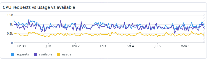
We see that our machines are reasonably sized for our needs, and that. This is not too surprising: engineers tend to err on the side of caution, and requests are increased whenever a bad event happens, but rarely decreased. We tried organizing “request days” where we would order pizzas for everyone and organize tuning workshops, but the benefits were minimal (if you ignore the pizzas 🍕), and never lasted because new features were implemented and new jobs deployed.

Most of our microservices are queue-based: they receive messages, process them, and send them to the next service. For those services, we can live with a little delay, and latency isn’t critical as long as it stays reasonable, which, for us, means under a few minutes. We would rather spare money and have a service be marginally slower than run it at peak capacity all the time.

We needed an automated, generic solution to optimize our requests and reduce our costs. Luckily, Kubernetes offers two such solutions out of the box: Vertical und Horizontal Pod Autoscalers. While seemingly simple, they are actually really difficult to implement properly.

This blog post recounts our experience, the traps we fell in, and the lessons we learned.

Please note that while we’ve added reminders when it made sense, some basic familiarity with VPAs and HPAs is assumed.

Vertical pod autoscalers

First, let’s discuss Vertical Pod Autoscalers. VPAs are Kubernetes native pod sizing tools. Given a pod and its CPU/memory usage history, the VPA Recommender computes a request recommendation. The VPA Updater then applies it to pods. These two components work together, and offer various configurations options. 

The Recommender has a lot of knobs you can twist to change how it computes its recommendation (more on that in a minute), but in Google Kubernetes Engine the Recommender is deployed in the control plane, and we cannot modify its configuration. We therefore expected it to work fine for our needs out of the box!

We already had VPAs in place, but they were configured to only suggest recommendations without actually modifying pods. 

We decided to switch all of our VPAs to the InPlace update mode, which would adapt pod requests without restarting them, and… confusion ensued. It worked well on some workloads, and not at all on others.

For example, see this workload, where the VPA was enabled at the start of the pink zone.

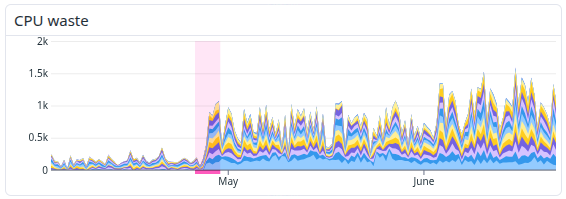
It got much worse. The question is: why?

Looking at the CPU usage of this workload, the VPA recommendation (in blue) appears ridiculously high compared to the average usage.

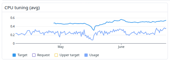
It took some time to understand why, but the reason is actually pretty simple! The default VPA looks at the pods CPU & memory usage history, plots the distribution for each of those, and then targets the 90th-percentile. It then adds a safety margin of 15%. In layman’s terms, this means it targets a request value such that the usage will stay below it for 90% of the time (and then adds a safety margin): it optimizes for load spikes.

Time series visualizers tend to aggregate samples by averaging them, and they don’t always store CPU usage as a distribution, which means what we’re charting here is not representative of what the VPA looks at.

Looking at the CPU max usage, i.e. taking the top of all usage spikes over the time period, we get a better understanding of the VPA recommendation.

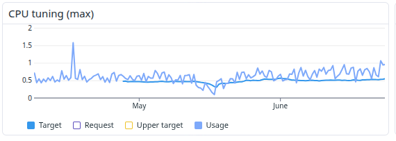
As expected, the recommendation is just under the top of all usage spikes.

Targeting the p90 is very conservative, and works well for extremely time sensitive workload. While we do have such workloads, most of our computing capacity is used to do complex data processing operations for which latency doesn’t matter that much. A delay of a few seconds throughout our entire pipeline isn’t the end of the world, and we would rather have workloads be throttled from time to time than constantly waste CPU cores.

Interestingly, we also need to differentiate between CPU and memory. Not having enough CPU is fine: the job will get slowed down, but it’ll get there eventually, since the kernel CFS fair-sharing guarantees it some amount of computing time. Not having enough memory is more annoying: under pressure the kernel will kill pods using more memory than they requested, incurring a significant restart/reprocessing cost. This means we can be much more aggressive with CPU than memory.

We run GKE (Google Kubernetes Engine) clusters, and, sadly, the default recommender is managed by GCP and isn’t configurable. However, it is possible and even easy to deploy a custom recommender with carefully selected parameters. VPAs can be configured to use this recommender, and the existing VPA chain (including the updater) will automatically switch to the new one. 

There is a Helm chart available, and modifying the default behavior is just a matter of passing the proper values to the extraArgs parameter:

• –recommender-name: the name of the recommender. This is what needs to be referenced in the VPA yaml
• –target-cpu-percentile: the targeted percentile (e.g. 0.5 is p50) for CPU recommendations
• –target-memory-percentile: the targeted percentile (same as above) for memory recommendations
• –recommendation-margin-fraction: the safety margin that’ll be added to the recommendation (default is 0.15, aka 15%)

Once the recommender is deployed and running, the VPA should reference it like this:

spec:

  recommenders:

  – name: recommender-frugal

The Updater component will then automatically use recommendations from the new recommender and proceed as before.

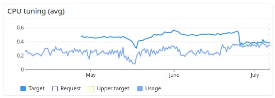
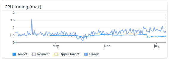
We decided to run a “frugal” recommender configured to target the p50 of CPU usage with no safety margin, applying it to all non time-sensitive recommendations. We deployed it at the end of June, and the effect was immediate. The graphs below show the VPA recommendation (“target”) is not much more aligned with the average usage (top graph) than the maximum usage (bottom graph). We are optimizing for the p50 (which is not the average, but is close in practice in this case) rather than the maximum, and reducing our costs in the process. Of course this is a trade-off: if all services suffer heavy load, we probably won’t have enough CPU to serve everyone, and pods will be temporarily throttled.

Going forward, we will probably maintain a small set of recommenders and select the best one depending on the workload type: default for critical, latency-sensitive workloads; frugal for most of our data processing services, etc.

What did we learn?

The default VPA recommender is very conservative in its recommendations, and heavily favors usage spikes. If your goal is to reduce costs and you can accept some throttling, this is not suitable. CPU recommendations can be much more aggressive than memory recommendations. Deploying a custom recommender is very easy, and does not require deploying the entire VPA ecosystem (updater, etc). 

Horizontal pod autoscalers

Now that we can rightsize pods, it’s time to step back and consider how many pods are actually needed. For stable workloads, we can study the load once and come up with a reasonable number, but our activity can be highly unpredictable, and we want our services to automatically adapt. The standard way to do this is to use a Horizontal Pod Autoscaler (HPA). HPAs automatically update the number of replicas required by a deployment based on a metric value and a target for this metric. The actual scaling formula is deceptively simple, but HPAs are full of pitfalls.

At CybelAngel we used to scale our services based on the size of the backlog of their input queues. That didn’t work well at all. 

For many services, this resulted in a surprising oscillating pattern: the HPA would alternately scale the deployment to its maximum, and then to its minimum.

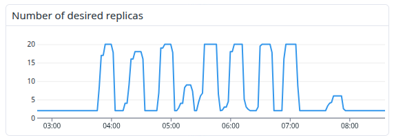
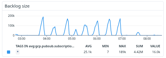
We spent a lot of time trying to understand what was going on, and our findings are summarized below.

Let’s first look at the scaling formula:

We have four different quantities in this formula:

• currentReplicas: current number of pods running for the service
• currentMetricValue: current value of the optimization metric (e.g. current CPU usage)
• desiredMetricValue: desired value of the optimization metric
• desiredReplicas: desired value of replicas, as computed by the HPA

The first two, currentReplicas und currentMetricValue are input for the HPA. desiredMetricValue is the control knob, and desiredReplicas is the output. 

HPAs evaluate this formula every 15 seconds by default, and update the desired number of replicas accordingly. If we ignore the rounding, we see it’s a basic cross-multiplication: if the metric is twice what it should be, the HPA doubles the number of replicas. 

This means scaling metrics must have the following properties:

• Move proportionally with the number of pods (if the number of pods doubles, the metric should halve)
• Update and reflect changes in the number of pods in less than 15 seconds
• Be related to the business metric we are trying to optimize

The default scaling metric, CPU usage, checks the first two boxes: CPU usage updates quickly and is, at first order, tied to the number of running pods. Sure, if you have a backlog you can double the number of pods and the CPU usage will remain high, but that’s a good thing, as it encodes the backlog size indirectly. 

Not all pods are CPU-bound though, which is why we were using the PubSub backlog size. But backlog size is a very bad scaling metric! The GCP metrics pipeline is ridiculously slow, and in our experience a sampled metric point can take up to 6 or even 8 minutes before it is available. Add a small processing delay to that (our HPAs pull data points from Datadog which itself polls GCP), and you are making decisions based on 10 minutes-old data. Worse, the backlog size metric is only sampled every minute, which means the HPA will make multiple decisions on the same metric point.

This explains the oscillating pattern we have been observing: the HPA input is essentially garbage, and isn’t updated nearly often enough. The HPA sees that the metric is above its target, and upscales accordingly. Fifteen seconds later the metric still hasn’t updated but the HPA wakes up, and scales up again. At some point we reach the maximum number of replicas, the backlog size decreases (because we have a ridiculous amount of replicas running, which also means we are reserving and wasting a ton of resources) and goes down to zero. The HPA sees the metric is now below the target, downscales… rinse and repeat. As our data scientists friends say, garbage in, garbage out.

We tried many metrics, including CPU usage, throughputs ratios (this one worked well but it doesn’t take the backlog into account) and eventually settled on exposing a custom metric tailored to our needs: the percentage of active threads from our processing thread pools. This is similar to CPU usage except it more accurately represents the pod’s processing capacity for steps that are not CPU-bound (threads are considered active during I/O too).

In our case, once we had a proper scaling metric we simply defined reasonable values for these two parameters, favoring scaling down (because, again, we can tolerate some delay). 

And… It worked! As soon as we deployed the HPAs using our new metric, the oscillating pattern disappeared.

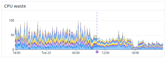
What did we learn?

The HPAs’ scaling algorithm is really simple but choosing a good metric isn’t. A good metric should be inversely proportional to the number of pods, reflect changes in less than 15 seconds, and accurately represent the pod’s capacity to process messages. Once the HPAs have a clean input, we can play with stabilisation windows and scaling policies to fine-tune their behaviour.

Schlussfolgerung

If we take a step back and look at the CPU waste on our example workload, the changes we made are really significant:

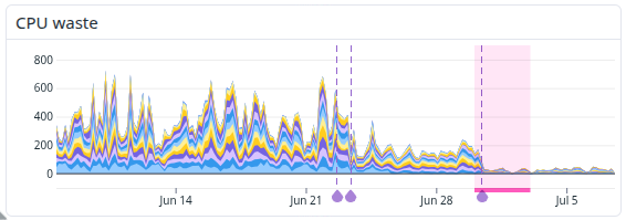
The first group of purple lines shows when we fixed our HPAs, second one (with the pink area) shows when we deployed the custom recommender for our VPAs. In total, that’s hundreds of CPU hours, and a lot of money saved without reducing performance! 

This blog post summarizes our findings, but understanding everything at play took us multiple days of investigation, testing, debugging, and analyzing our metrics. Proper scaling is hard. You need both functional VPAs, with a recommender matching your latency and risk appetite goals, and functional HPAs, acting on a properly defined metric tied to your business goals. Only at these conditions do you get the right amount of rightly sized pods.

We hope this blog post has been an interesting read, and that these tips will be helpful. As for us, we are going to apply our findings to our biggest workloads, and we think we will be able to significantly reduce our cloud bill.